MO-201 Real Exam Questions

Microsoft Excel Expert (Excel and Excel 2019)

24 questions available · Page 1 of 3

Updated Exam DumpsVerified AnswersPass Guarantee

Get Complete Exam Dumps
Question 1 Lab simulation

Simulation

From the "Employees" worksheet, create a macro named "Header". Store the macro in the current workbook. Configure the macro to insert the "Sheet Name" in the left header cell of the active page and the "Page Number" in the right header cell.

Show answer and explanation

The Developer tab isn't displayed by default, but you can add it to the ribbon.

On the File tab, go to Options > Customize Ribbon. Under Customize the Ribbon and under Main Tabs, select the Developer check box.

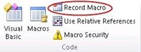
Record a macro 1. In the Code group on the Developer tab, click Record Macro.
2. Optionally, enter a name for the macro in the Macro name box and a description in the Description box, and then click OK to start recording.
3. Select Page layout from the Ribbon and expand Page Setup.
4. Select the Header/Footer tab and click Custom Header.
5. In the Left section, click the Insert Sheet Name button.
6. In the Right section, click the Insert Page Number button.
7. Click OK. Then click OK again.
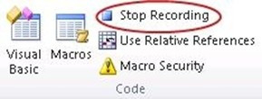
8. On the Developer tab, click Stop Recording.
9. On the Developer tab, click Macros to view the available Macros.
10. Select the Macro and click Run.
Question 2 Lab simulation

Simulation

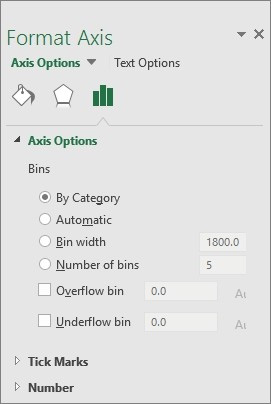
On the "New Products" worksheet, create a Histogram chart that shows the "Retail Price" of the products in bins with widths of $10.
The chart size and position do not matter.

Show answer and explanation

1. Select your data.
2. Click Insert > Insert Statistic Chart > Histogram.
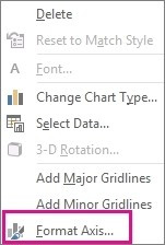
3. Right-click the horizontal axis of the chart, click Format Axis, and then click Axis Options.

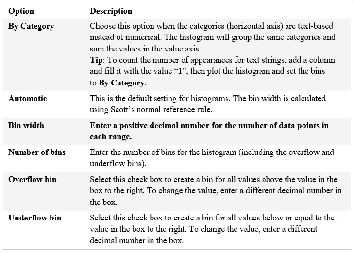
4. Use the information in the following table to decide which options you want to set in the Format Axis task pane.

Question 3 Lab simulation

Simulation

On the "New Titles" worksheet, for cells E4:E24, create and apply a custom number format that displays the dates in the format "2020 January 01".

Show answer and explanation

1. Select the cells you want to format.
2. Press CTRL+1.
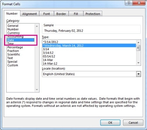
3. In the Format Cells box, click the Number tab.
4. In the Category list, click Date, and then choose a date format you want in Type. You can adjust this format in the last step below.

5. Go back to the Category list, and choose Custom. Under Type, you'll see the format code for the date format you chose in the previous step. The built-in date format can't be changed, so don't worry about messing it up. The changes you make will only apply to the custom format you're creating.
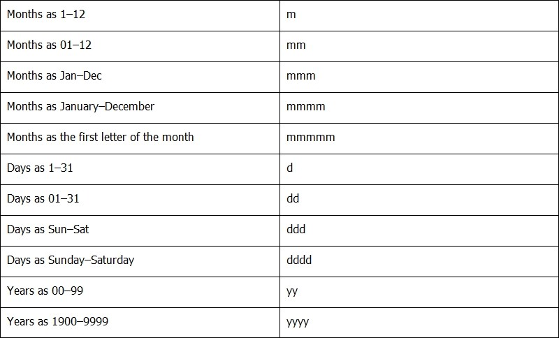
6. In the Type box, make the changes you want using code from the table below. In our case, yyyy mmmm dd.

7. Click OK.

Question 4 Lab simulation

Simulation

On the "Sales Conference" worksheet, configure cells A4:A12 to allow only whole numbers from 1 to 9.

Otherwise, display a Stop error with the title "Invalid" and the message "1 to 9".

Show answer and explanation

1. Select the cell(s) you want to create a rule for.

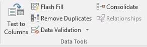
2. Select Data >Data Validation.
3. On the Settings tab, under Allow, select an option:
Whole Number - to restrict the cell to accept only whole numbers. Decimal - to restrict the cell to accept only decimal numbers.
List - to pick data from the drop-down list.
Date - to restrict the cell to accept only date. Time - to restrict the cell to accept only time. Text Length - to restrict the length of the text.
Custom ?for custom formula.
4. Under Data, select a condition:
between
not between
equal to
not equal to
greater than
less than greater than or equal to less than or equal to
5. On the Settings tab, under Allow, select an option:
6. Set the other required values, based on what you chose for Allow and Data. For example, if you select between, then select the Minimum: and Maximum: values for the cell(s).
7. Select the Ignore blank checkbox if you want to ignore blank spaces.
8. If you want to add a Title and message for your rule, select the Input Message tab, and then type a title and input message.
9. Select the Show input message when cell is selected checkbox to display the message when the user selects or hovers over the selected cell(s).
10. Select OK.Now, if the user tries to enter a value that is not valid, a pop-up appears with the message, "This value doesn't match the data validation restrictions for this cell."

Question 5 Lab simulation

Simulation

This project has only one task.

Configure Excel to automatically evaluate formulas only when a workbook is saved, and not each time data changes.

Show answer and explanation

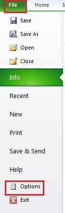
1. Click "File" in the ribbon.

2. And then click "Options".
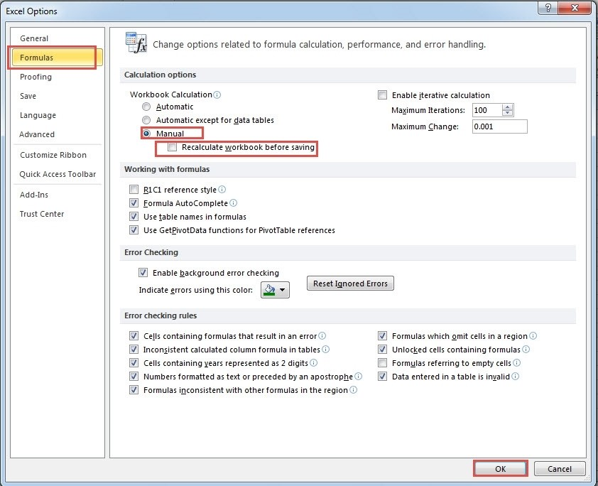
3. In the "Excel Options", choose the "Formulas".
4. And then in the "Calculation Options", check the option "Manual".
5. Check the Recalculate workbook before saving option.

6. And then click "OK" in the window.
7. Next save the workbook.

Question 6 Lab simulation

Simulation

On the "Royalty Analysis" worksheet, add the "Title ID" field as a PivotChart filter. Apply the filter to the chart to display only results for title ID "CO20".

Show answer and explanation

In the PivotTable Field list, click on the field that you want to use as a Report Filter.
Drag the field into the Filters box.
On the worksheet, Excel adds the selected field to the top of the pivot table, with the item (All) showing.
The values in the pivot table do not change. Click the Report Filter's drop-down arrow, to see a list of items in the field.
Click on an item to select it, and click OK.

Question 7 Lab simulation

Simulation

On the "Employees" worksheet, in cell F4, enter a formula that returns the employee's bonus from the "Years of Service Bonus" table.

Adjust the formula and then copy it to cells F5:F19.

Show answer and explanation

Select cell F4.
Enter the following formula:=INDEX($I$2:$I$7,MATCH(B4,$H$2:$H$7,1),1) Press Enter.

Question 8 Lab simulation

Simulation

On the "Plan Analysis" worksheet, modify the PivotTable to group the data by the values in the "Full Package Price" column. Group the values in steps of 100 beginning at 0 and ending at 200.

Show answer and explanation

In the PivotTable, right-click a value and select Group.

In the Grouping box, select Starting at and Ending at checkboxes, and edit the values if needed. (0 and
200 respectively)

Under By, enter a number that specifies the interval for each group. (100)

Select OK.

Question 9 Lab simulation

Simulation

On the "Volunteer Analysis" chart sheet, drill down into the data to display the number of volunteer hours for each month.

Show answer and explanation

If a chart has multiple fields in the Axis box, you set it to show levels and you see only one level at a time, starting with the top level.
To enable drill-down, access the Design tab > Show Levels > Enable Drill Down One Level at a Time.
if you double-click on one of the bars, you will see the bars for the underlying data.

Question 10 Lab simulation

Simulation

On the "Regional Sales" worksheet, modify the PivotTable to display the "Territory" rows within each region.

Show answer and explanation

Click anywhere in the PivotTable to display the Field List. Check the box next to Territory, and it should be added to the Rows area by default. The PivotTable should now be displaying Territory rows within each region.